37 posts tagged with "Edge Computing"

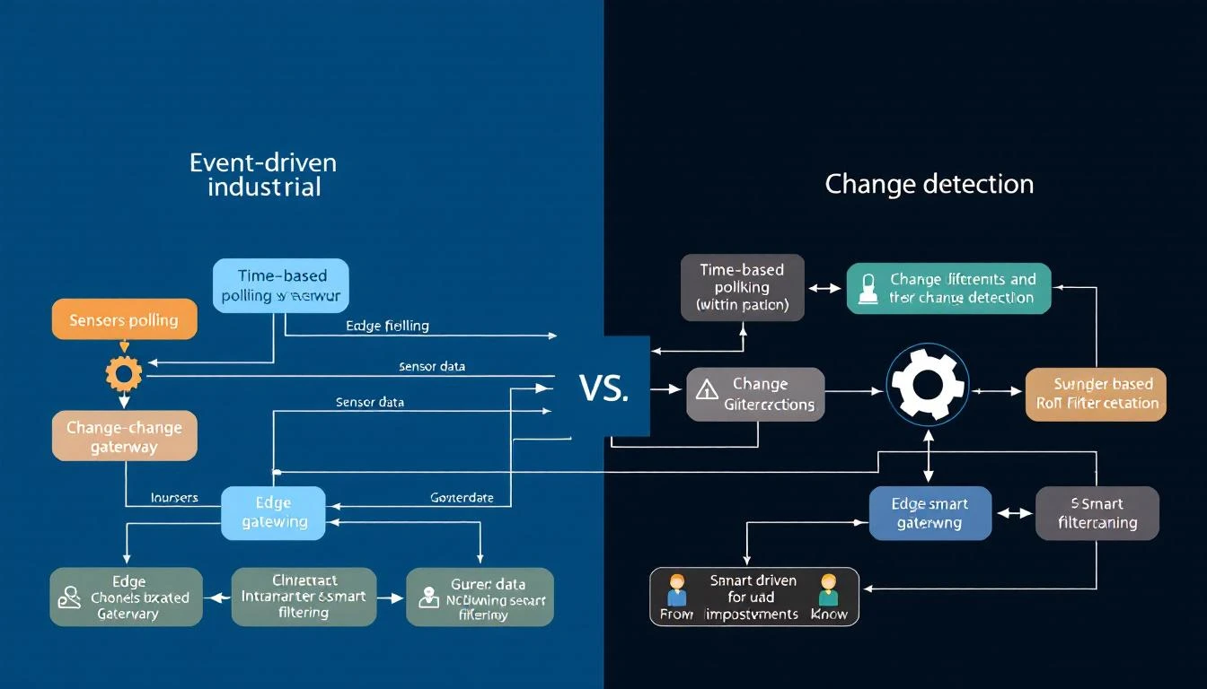
Most IIoT platforms treat every data point as equal. They poll each tag on a fixed schedule, blast everything to the cloud, and let someone else figure out what matters. That approach works fine when you have ten tags. It collapses when you have ten thousand.

Production-grade edge systems take a fundamentally different approach: they model relationships between tags — parent-child dependencies, calculated values derived from raw registers, and event-driven reads that fire only when upstream conditions change. The result is dramatically less bus traffic, lower latency on the signals that matter, and a data architecture that mirrors how the physical process actually works.

This article is a deep technical guide to building these hierarchical tag architectures from the ground up.

The Problem with Flat Polling​

In a traditional SCADA or IIoT setup, the edge gateway maintains a flat list of tags. Each tag has an address and a polling interval:

Tag: Barrel_Temperature    Address: 40001    Interval: 1s
Tag: Screw_Speed           Address: 40002    Interval: 1s
Tag: Mold_Pressure         Address: 40003    Interval: 1s
Tag: Machine_State         Address: 40010    Interval: 1s
Tag: Alarm_Word_1          Address: 40020    Interval: 1s
Tag: Alarm_Word_2          Address: 40021    Interval: 1s

Every second, the gateway reads every tag — regardless of whether anything changed. This creates three problems:

1. Bus saturation on serial links. A Modbus RTU link at 9600 baud can handle roughly 10–15 register reads per second. With 200 tags at 1-second intervals, you're mathematically guaranteed to fall behind.

2. Wasted bandwidth to the cloud. If barrel temperature hasn't changed in 30 seconds, you're uploading the same value 30 times. At $0.005 per MQTT message on most cloud IoT services, that adds up.

3. Missing the events that matter. When everything polls at the same rate, a critical alarm state change gets the same priority as a temperature reading that hasn't moved in an hour.

Introducing Tag Hierarchies​

A dependent tag architecture introduces three concepts:

1. Parent-Child Dependencies​

A dependent tag is one that only gets read when its parent tag's value changes. Consider a machine status word. When the status word changes from "Running" to "Fault," you want to immediately read all the associated diagnostic registers. When the status word hasn't changed, those diagnostic registers are irrelevant.

# Conceptual configuration
parent_tag:
  name: machine_status_word
  address: 40010
  interval: 1s
  compare: true
  dependent_tags:
    - name: fault_code
      address: 40011
    - name: fault_timestamp
      address: 40012-40013
    - name: last_setpoint
      address: 40014

When machine_status_word changes, the edge daemon immediately performs a forced read of all three dependent tags and delivers them in the same telemetry group — with the same timestamp. This guarantees temporal coherence: the fault code, timestamp, and last setpoint all share the exact timestamp of the state change that triggered them.

2. Calculated Tags​

A calculated tag is a virtual data point derived from a parent tag's raw value through bitwise operations. The most common use case: decoding packed alarm words.

Industrial PLCs frequently pack 16 boolean alarms into a single 16-bit register. Rather than polling 16 separate coil addresses (which requires 16 Modbus transactions), you read one holding register and extract each bit:

Alarm_Word_1 (uint16 at 40020):
  Bit 0 → High Temperature Alarm
  Bit 1 → Low Pressure Alarm
  Bit 2 → Motor Overload
  Bit 3 → Emergency Stop Active
  ...
  Bit 15 → Communication Fault

A well-designed edge gateway handles this decomposition at the edge:

parent_tag:
  name: alarm_word_1
  address: 40020
  type: uint16
  interval: 1s
  compare: true       # Only process when value changes
  do_not_batch: true  # Deliver immediately — don't wait for batch timeout
  calculated_tags:
    - name: high_temp_alarm
      type: bool
      shift: 0
      mask: 0x01
    - name: low_pressure_alarm
      type: bool
      shift: 1
      mask: 0x01
    - name: motor_overload
      type: bool
      shift: 2
      mask: 0x01
    - name: estop_active
      type: bool
      shift: 3
      mask: 0x01

The beauty of this approach:

• One Modbus read instead of sixteen
• Zero cloud processing — the edge already decomposed the alarm word into named boolean tags
• Change-driven delivery — if the alarm word hasn't changed, nothing gets sent. When bit 2 flips from 0 to 1, only the changed calculated tags get delivered.

3. Comparison-Based Delivery​

The compare flag on a tag definition tells the edge daemon to track the last-known value and suppress delivery when the new value matches. This is distinct from a polling interval — the tag still gets read on schedule, but the value only gets delivered when it changes.

This is particularly powerful for:

• Status words and mode registers that change infrequently
• Alarm bits where you care about transitions, not steady state
• Setpoint registers that only change when an operator makes an adjustment

A well-implemented comparison handles type-aware equality. Comparing two float values with bitwise equality is fine for PLC registers (they're IEEE 754 representations read directly from memory — no floating-point arithmetic involved). Comparing two uint16 values is straightforward. The edge daemon should store the raw bytes, not a converted representation.

Register Grouping: The Foundation​

Before dependent tags can work efficiently, the underlying polling engine needs contiguous register grouping. This is the practice of combining multiple tags into a single Modbus read request when their addresses are adjacent.

Consider these five tags:

Tag A: addr 40001, type uint16  (1 register)
Tag B: addr 40002, type uint16  (1 register)
Tag C: addr 40003, type float   (2 registers)
Tag D: addr 40005, type uint16  (1 register)
Tag E: addr 40010, type uint16  (1 register)  ← gap

An intelligent polling engine groups A through D into a single Read Holding Registers call: start address 40001, quantity 5. Tag E starts a new group because there's a 5-register gap.

The grouping rules are:

1. Same function code. You can't combine holding registers (FC03) with input registers (FC04) in one read.
2. Contiguous addresses. Any gap breaks the group.
3. Same polling interval. A tag polling at 1s and a tag polling at 60s shouldn't be in the same group.
4. Maximum group size. The Modbus spec limits a single read to 125 registers (some devices impose lower limits — 50 is a safe practical maximum).

After the bulk read returns, the edge daemon dispatches individual register values to each tag definition, handling type conversion per tag (uint16, int16, float from two consecutive registers, etc.).

The 32-Bit Float Problem​

When a tag spans two Modbus registers (common for 32-bit integers and IEEE 754 floats), the edge daemon must handle word ordering. Some PLCs store the high word first (big-endian), others store the low word first (little-endian). A typical edge system stores the raw register pair and then calls the appropriate conversion:

• Big-endian (AB CD): value = (register[0] << 16) | register[1]
• Little-endian (CD AB): value = (register[1] << 16) | register[0]

For IEEE 754 floats, the 32-bit integer is reinterpreted as a floating-point value. Getting this wrong produces garbage data — a common source of "the numbers look random" support tickets.

Architecture: Tying It Together​

Here's how a production edge system processes a single polling cycle with dependent tags:

1. Start timestamp group (T = now)
2. For each tag in the poll list:
   a. Check if interval has elapsed since last read
   b. If not due, skip (but check if it's part of a contiguous group)
   c. Read tag (or group of tags) from PLC
   d. If compare=true and value unchanged: skip delivery
   e. If compare=true and value changed:
      i.   Deliver value (batched or immediate)
      ii.  If tag has calculated_tags: compute each one, deliver
      iii. If tag has dependent_tags:
           - Finalize current batch group
           - Force-read all dependent tags (recursive)
           - Start new batch group
   f. Update last-known value and last-read timestamp
3. Finalize timestamp group

The critical detail is step (e)(iii): when a parent tag triggers a dependent read, the current batch group gets finalized and the dependent tags are read in a forced mode (ignoring their individual interval timers). This ensures the dependent values reflect the state at the moment of the parent's change, not some future polling cycle.

Practical Considerations​

Serial Link Timing​

On Modbus RTU, the 3.5-character silent interval between frames is mandatory. At 9600 baud with 8N1 encoding, one character takes ~1.04ms, so the minimum inter-frame gap is ~3.64ms. With a typical request frame of 8 bytes and a response frame of 5 + 2*N bytes (for N registers), a single read of 10 registers takes approximately:

Request:    8 bytes × 1.04ms = 8.3ms
Turnaround: ~3.5ms (device processing)
Response:   (5 + 20) bytes × 1.04ms = 26ms
Gap:        3.64ms
Total:      ~41.4ms per read

This means you can fit roughly 24 read operations per second on a 9600-baud link. If you're polling 150 tags with 1-second intervals, grouping is not optional — it's survival.

Alarm Tag Design​

For alarm words, always configure:

• compare: true — only deliver when an alarm state changes
• do_not_batch: true — bypass the batch timeout and deliver immediately
• interval: 1 (1 second) — poll frequently to catch transient alarms

Process variables like temperatures and pressures can safely use longer intervals (30–60 seconds) with compare: false since trending data benefits from regular samples.

Avoiding Circular Dependencies​

If Tag A is dependent on Tag B, and Tag B is dependent on Tag A, you'll create an infinite recursion in the read loop. Production systems guard against this by either:

• Limiting dependency depth (typically 1–2 levels)
• Tracking a "reading" flag to prevent re-entry
• Flattening the graph at configuration parse time

Hourly Full-Refresh​

Even with change-driven delivery, it's good practice to force-read and deliver all tags at least once per hour. This catches any edge cases where a value changed but the change was missed (e.g., a brief network hiccup that caused a read failure during the exact moment of change). A simple approach: track the hour boundary and reset the "already read" flag on all tags when the hour rolls over.

How machineCDN Handles Tag Hierarchies​

machineCDN's edge infrastructure supports all three relationship types natively. When you configure a device in the platform, you define parent-child dependencies, calculated alarm bits, and comparison-based delivery in the device configuration — no custom scripting required.

The platform's edge daemon handles contiguous register grouping automatically, supports both EtherNet/IP and Modbus (TCP and RTU) from the same configuration model, and provides dual-format batch delivery (JSON for debugging, binary for bandwidth efficiency). Alarm tags are delivered immediately outside the batch cycle, ensuring sub-second alert latency even when the batch timeout is set to 30 seconds.

For teams managing fleets of machines across multiple plants, this means the tag architecture you define once gets deployed consistently to every edge gateway — whether it's monitoring a chiller system with 160+ process variables or a simple TCU with 20 tags.

Key Takeaways​

1. Model relationships, not just addresses. Tags have dependencies that mirror the physical process. Your data architecture should reflect that.
2. Use comparison to suppress noise. A status word that hasn't changed in 6 hours doesn't need 21,600 duplicate deliveries.
3. Calculated tags eliminate cloud processing. Decompose packed alarm words at the edge — one Modbus read becomes 16 named boolean signals.
4. Dependent reads guarantee temporal coherence. When a parent changes, all children are read with the same timestamp.
5. Group contiguous registers ruthlessly. On serial links, the difference between grouped and ungrouped reads is the difference between working and not working.

The flat-list polling model was fine for SCADA systems monitoring 50 tags on a single HMI. For IIoT platforms handling thousands of data points across fleets of machines, hierarchical tag architectures aren't an optimization — they're the foundation.

Most IIoT deployments start the same way: poll every PLC register every second, serialize all values to JSON, and push everything to the cloud over MQTT. It works — until your cellular data bill arrives, or your broker starts choking on 500,000 messages per day from a single gateway, or you realize that 95% of those messages contain values that haven't changed since the last read.

The reality of industrial data is that most values don't change most of the time. A chiller's tank temperature drifts by a fraction of a degree per minute. A blender's motor state is "running" for 8 hours straight. A conveyor's alarm register reads zero all day — until the instant it doesn't, and that instant matters more than the previous 86,400 identical readings.

This guide covers a smarter approach: event-driven tag delivery, where the edge gateway reads at regular intervals but only transmits when something actually changes — and when something does change, it can trigger reads of related tags for complete context.

The Problem with Fixed-Interval Everything​

Let's quantify the waste. Consider a typical industrial chiller with 10 compressor circuits, each exposing 16 process tags (temperatures, pressures, flow rates) and 3 alarm registers:

Tags per circuit:  16 process + 3 alarm = 19 tags
Total tags:        10 circuits × 19 = 190 tags
Poll interval:     All at 1 second

At JSON format with timestamp, tag ID, and value, each data point is roughly 50 bytes. Per second, that's:

190 tags × 50 bytes = 9,500 bytes/second
= 570 KB/minute
= 34.2 MB/hour
= 821 MB/day

Over a cellular connection at $5/GB, that's $4.10/day per chiller — just for data that's overwhelmingly identical to what was sent one second ago.

Now let's separate the tags by their actual change frequency:

Those 30 alarm registers — 15.8% of your data volume — change roughly 5 times per day. You're transmitting them 86,400 times. That's a 17,280x overhead on alarm data.

The Three Pillars of Event-Driven Delivery​

A well-designed edge gateway implements three complementary strategies:

1. Compare-on-Read (Change Detection)​

The simplest optimization: after reading a tag value from the PLC, compare it against the last transmitted value. If it hasn't changed, don't send it.

The implementation is straightforward:

# Pseudocode — NOT from any specific codebase
def should_deliver(tag, new_value, new_status):
    # Always deliver the first reading
    if not tag.has_been_read:
        return True
    
    # Always deliver on status change (device went offline/online)
    if tag.last_status != new_status:
        return True
    
    # Compare values if compare flag is enabled
    if tag.compare_enabled:
        if tag.last_value != new_value:
            return True
        return False  # Value unchanged, skip
    
    # If compare disabled, always deliver
    return True

Which tags should use change detection?

• Alarm/status registers: Always. These are event-driven by nature — you need the transitions, not the steady state.
• Digital I/O: Always. Binary values either changed or they didn't.
• Configuration registers: Always. Software version numbers, setpoints, and device parameters change rarely.
• Temperatures and pressures: Situational. If the process is stable, most readings are identical. But if you need trending data for analytics, you may want periodic delivery regardless.
• Counter registers: Never. Counters increment continuously — every reading is "different" — and you need the raw values for accurate rate calculations.

The gotcha with floating-point comparison: Comparing IEEE 754 floats for exact equality is unreliable due to rounding. For float-typed tags, use a deadband:

# Apply deadband for float comparison
def float_changed(old_val, new_val, deadband=0.1):
    return abs(new_val - old_val) > deadband

A temperature deadband of 0.1°F means you'll transmit when the temperature moves meaningfully, but ignore sensor noise.

2. Dependent Tags (Contextual Reads)​

Here's where event-driven delivery gets powerful. Consider this scenario:

A chiller's compressor status word is a 16-bit register where each bit represents a different state: running, loaded, alarm, lockout, etc. You poll this register every second with change detection enabled. When bit 7 flips from 0 to 1 (alarm condition), you need more than just the status word — you need the discharge pressure, suction temperature, refrigerant level, and superheat at that exact moment to diagnose the alarm.

The solution: dependent tag chains. When a parent tag's value changes, the gateway immediately triggers a forced read of all dependent tags, delivering the complete snapshot:

Parent Tag:    Compressor Status Word (polled every 1s, compare=true)
Dependent Tags:
  ├── Discharge Pressure (read only when status changes)
  ├── Suction Temperature (read only when status changes)
  ├── Refrigerant Liquid Temp (read only when status changes)
  ├── Superheat (read only when status changes)
  └── Subcool (read only when status changes)

In normal operation, the gateway reads only the status word — one register per second per compressor. When the status word changes, it reads 6 registers total and delivers them as a single timestamped group. The result:

• Steady state: 1 register/second → 50 bytes/second
• Event triggered: 6 registers at once → 300 bytes (once, at the moment of change)
• vs. polling everything: 6 registers/second → 300 bytes/second (continuously)

Bandwidth savings: 99.8% during steady state, with zero data loss at the moment that matters.

3. Calculated Tags (Bit-Level Decomposition)​

Industrial PLCs often pack multiple boolean signals into a single 16-bit or 32-bit "status word" or "alarm word." Each bit has a specific meaning defined in the PLC program documentation:

Alarm Word (uint16):
  Bit 0:  High Temperature Alarm
  Bit 1:  Low Pressure Alarm
  Bit 2:  Flow Switch Fault
  Bit 3:  Motor Overload
  Bit 4:  Sensor Open Circuit
  Bit 5:  Communication Fault
  Bits 6-15: Reserved

A naive approach reads the entire word and sends it to the cloud, leaving the bit-level parsing to the backend. A better approach: the edge gateway decomposes the word into individual boolean tags at read time.

The gateway reads the parent tag (the alarm word), and for each calculated tag, it applies a shift and mask operation to extract the individual bit:

Individual Alarm = (alarm_word >> bit_position) & mask

Each calculated tag gets its own change detection. So when Bit 2 (Flow Switch Fault) transitions from 0 to 1, the gateway transmits only that specific alarm — not the entire word, and not any unchanged bits.

Why this matters at scale: A 10-circuit chiller has 30 alarm registers (3 per circuit), each 16 bits wide. That's 480 individual alarm conditions. Without bit decomposition, a single bit flip in one register transmits all 30 registers (because the polling cycle doesn't know which register changed). With calculated tags, only the one changed boolean is transmitted.

Batching: Grouping Efficiency​

Even with change detection, transmitting each changed tag as an individual MQTT message creates excessive overhead. MQTT headers, TLS framing, and TCP acknowledgments add 80-100 bytes of overhead per message. A 50-byte tag value in a 130-byte envelope is 62% overhead.

The solution: time-bounded batching. The gateway accumulates changed tag values into a batch, then transmits the batch when either:

1. The batch reaches a size threshold (e.g., 4KB of accumulated data)
2. A time limit expires (e.g., 10-30 seconds since the batch started collecting)

The batch structure groups values by timestamp:

{
  "groups": [
    {
      "ts": 1709335200,
      "device_type": 1018,
      "serial_number": 2411001,
      "values": [
        {"id": 1, "values": [245]},
        {"id": 6, "values": [187]},
        {"id": 7, "values": [42]}
      ]
    }
  ]
}

Critical exception: alarm tags bypass batching. When a status register changes, you don't want the alarm notification sitting in a batch buffer for 30 seconds. Alarm tags should be marked as do_not_batch — they're serialized and transmitted immediately as individual messages with QoS 1 delivery confirmation.

This creates a two-tier delivery system:

Binary vs. JSON: The Encoding Decision​

The batch payload format has a surprisingly large impact on bandwidth. Consider a batch with 50 tag values:

JSON format:

{"groups":[{"ts":1709335200,"device_type":1018,"serial_number":2411001,"values":[{"id":1,"values":[245]},{"id":2,"values":[187]},...]}]}

Typical size: 2,500-3,000 bytes for 50 values

Binary format:

Header:     1 byte  (magic byte 0xF7)
Group count: 4 bytes
Per group:
  Timestamp:      4 bytes
  Device type:    2 bytes
  Serial number:  4 bytes
  Value count:    4 bytes
  Per value:
    Tag ID:       2 bytes
    Status:       1 byte
    Value count:  1 byte
    Value size:   1 byte (1=bool/int8, 2=int16, 4=int32/float)
    Values:       1-4 bytes each

Typical size: 400-600 bytes for 50 values

That's a 5-7x reduction — from 3KB to ~500 bytes per batch. Over cellular, this is transformative. A device that transmits 34 MB/day in JSON drops to 5-7 MB/day in binary, before even accounting for change detection.

The trade-off: binary payloads require a schema-aware decoder on the cloud side. Both the gateway and the backend must agree on the encoding format. In practice, most production IIoT platforms use binary encoding for device-to-cloud telemetry and JSON for cloud-to-device commands (where human readability matters and message volume is low).

The Hourly Reset: Catching Drift​

One subtle problem with pure change detection: if a value drifts by tiny increments — each below the comparison threshold — the cloud's cached value can slowly diverge from reality. After hours of accumulated micro-drift, the dashboard shows 72.3°F while the actual temperature is 74.1°F.

The solution: periodic forced reads. Every hour (or at another configurable interval), the gateway resets all "read once" flags and forces a complete read of every tag, delivering all current values regardless of change. This acts as a synchronization pulse that corrects any accumulated drift and confirms that all devices are still online.

The hourly reset typically generates one large batch — a snapshot of all 190 tags — adding roughly 10-15KB once per hour. That's negligible compared to the savings from change detection during the other 3,599 seconds.

Quantifying the Savings​

Let's revisit our 10-circuit chiller example with event-driven delivery:

Before (fixed interval, everything at 1s):

190 tags × 86,400 seconds × 50 bytes = 821 MB/day

After (event-driven with change detection):

Process values: 160 tags × avg 2 changes/min × 1440 min × 50 bytes = 23 MB/day
Alarm bits:     30 tags × avg 5 changes/day × 50 bytes            = 7.5 KB/day
Hourly resets:  190 tags × 24 resets × 50 bytes                   = 228 KB/day
Overhead (headers, keepalives):                                   ≈ 2 MB/day
──────────────────────────────────────────────────────
Total:                                                            ≈ 25.2 MB/day

With binary encoding instead of JSON:

≈ 25.2 MB/day ÷ 5.5 (binary compression) ≈ 4.6 MB/day

Net reduction: 821 MB → 4.6 MB = 99.4% bandwidth savings.

On a $5/GB cellular plan, that's $4.10/day → $0.02/day per chiller.

Implementation Checklist​

If you're building or evaluating an edge gateway for event-driven tag delivery, here's what to look for:

• Per-tag compare flag — Can you enable/disable change detection per tag?
• Per-tag polling interval — Can fast-changing and slow-changing tags have different read rates?
• Dependent tag chains — Can a parent tag's change trigger reads of related tags?
• Bit-level calculated tags — Can alarm words be decomposed into individual booleans?
• Bypass batching for alarms — Are alarm tags delivered immediately, bypassing the batch buffer?
• Binary encoding option — Can the gateway serialize in binary instead of JSON?
• Periodic forced sync — Does the gateway do hourly (or configurable) full reads?
• Link state tracking — Is device online/offline status treated as a first-class event?

How machineCDN Handles Event-Driven Delivery​

machineCDN's edge gateway implements all of these strategies natively. Every tag in the device configuration carries its own polling interval, change detection flag, and batch/immediate delivery preference. Alarm registers are automatically configured for 1-second polling with change detection and immediate delivery. Process values use configurable intervals with batched transmission. The gateway supports both JSON and compact binary encoding, with automatic store-and-forward buffering that retains data through connectivity outages.

The result: plants running machineCDN gateways over cellular connections typically see 95-99% lower data volumes compared to naive fixed-interval polling — without losing a single alarm event or meaningful process change.

Tired of paying for the same unchanged data point 86,400 times a day? machineCDN delivers only the data that matters — alarms instantly, process values on change, with full periodic sync. See how much bandwidth you can save.

The edge gateway is where the factory floor meets the cloud. It's the device — and the software running on it — that reads data from your PLCs, sensors, and controllers, processes it locally, and transmits it to cloud platforms for analytics, monitoring, and predictive maintenance.

In 2026, the edge gateway market has matured significantly. You no longer need to build custom solutions with Raspberry Pis and Python scripts. Purpose-built industrial edge gateway software handles protocol translation, data buffering, security, and cloud connectivity out of the box. But the options range from bare-metal connectivity platforms to full IIoT suites that include the edge as just one component.

Here's how to evaluate edge gateway software and which platforms deliver the most value for manufacturing environments.

In industrial IoT, the MQTT connection between an edge gateway and the cloud isn't just another network link — it's the lifeline that carries every sensor reading, every alarm event, and every machine heartbeat from the factory floor to the platform where decisions get made. When that connection fails (and it will), the difference between losing data and delivering it reliably comes down to how well you've designed your resilience patterns.

This guide covers the engineering patterns that make MQTT connections production-hardened for industrial telemetry — the kind of patterns that emerge only after years of operating edge devices in factories with unreliable cellular connections, expired certificates, and firmware updates that reboot network interfaces at 2 AM.

The Industrial MQTT Reliability Challenge​

Enterprise MQTT (monitoring dashboards, chat apps, consumer IoT) can tolerate occasional message loss. Industrial MQTT cannot. Here's why:

• A single missed alarm could mean a $200,000 compressor failure goes undetected
• Regulatory compliance may require continuous data records with no gaps
• Production analytics (OEE, downtime tracking) become meaningless with data holes
• Edge gateways operate unattended for months or years — there's nobody to restart the process

The standard MQTT client libraries provide reconnection, but reconnection alone isn't resilience. True resilience means:

1. Data generated during disconnection is preserved
2. Reconnection happens without blocking data acquisition
3. Authentication tokens are refreshed before they expire
4. The system detects and recovers from "zombie connections" (TCP says connected, but no data flows)
5. All of this works on devices with 32MB of RAM running on cellular networks

Asynchronous Connection Architecture​

The first and most important pattern: never let MQTT connection attempts block your data acquisition loop.

The Problem with Synchronous Connect​

A synchronous mqtt_connect() call blocks until it either succeeds or times out. On a cellular network with DNS issues, this can take 30–60 seconds. During that time, your edge device isn't reading any PLCs, which means:

• Lost data points during the connection attempt
• Stale data in the PLC's scan buffer
• Potential PLC communication timeouts if you miss polling windows

The Async Pattern​

The production-proven pattern separates the connection lifecycle into its own thread:

Main Thread:                    Connection Thread:
┌─────────────┐                ┌──────────────────┐
│ Read PLCs   │                │ Wait for signal   │
│ Batch data  │──signal───────>│ Connect async     │
│ Buffer data │                │ Set callbacks      │
│ Continue... │<──callback─────│ Report status      │
└─────────────┘                └──────────────────┘

Key design decisions:

1. Use a semaphore pair to coordinate: one "job ready" semaphore and one "thread idle" semaphore. The main thread only signals a new connection attempt if the connection thread is idle (try-wait on the idle semaphore).

2. Connection thread is long-lived — it starts at boot and runs forever, waiting for connection signals. Don't create/destroy threads for each connection attempt; the overhead on embedded Linux systems is significant.

3. Never block the main thread waiting for connection. If the connection thread is busy with a previous attempt, skip and try again on the next cycle.

// Pseudocode for async connection pattern
void connection_thread() {
    while (true) {
        wait(job_semaphore);         // Block until signaled
        
        result = mqtt_connect_async(host, port, keepalive=60);
        if (result != SUCCESS) {
            log("Connection attempt failed: %d", result);
        }
        
        post(idle_semaphore);        // Signal that we're done
    }
}

void main_loop() {
    while (true) {
        read_plc_data();
        batch_and_buffer_data();
        
        if (!mqtt_connected && try_wait(idle_semaphore)) {
            // Connection thread is idle — kick off new attempt
            post(job_semaphore);
        }
    }
}

Reconnection Delay​

After a disconnection, don't immediately hammer the broker with reconnection attempts:

• Fixed delay: 5 seconds between attempts works well for most industrial scenarios
• Don't use exponential backoff for industrial MQTT — unlike consumer apps where millions of clients might storm a broker simultaneously, your edge gateway is one device connecting to one endpoint. A constant 5-second retry gets you reconnected faster than exponential backoff without creating meaningful load.
• Disable jitter — again, you're not protecting against thundering herd. Get connected as fast as reliably possible.

Page-Based Output Buffering​

The output buffer is where resilience lives. When MQTT is disconnected, data keeps flowing from PLCs. Without proper buffering, that data is lost.

Buffer Architecture​

The most robust pattern for embedded systems uses a page-based ring buffer:

┌──────────┐ ┌──────────┐ ┌──────────┐ ┌──────────┐
│  Page 0  │ │  Page 1  │ │  Page 2  │ │  Page 3  │
│ [filled] │ │ [filling]│ │  [free]  │ │  [free]  │
│  sent ✓  │ │  ← write │ │          │ │          │
└──────────┘ └──────────┘ └──────────┘ └──────────┘
     ↑ read

Three page states:

• Free pages: Available for new data
• Work page: Currently being written to by the data acquisition loop
• Used pages: Filled with data, waiting to be sent

How it flows:

1. Data arrives from the batch layer → written to the current work page
2. When the work page is full → moved to the used pages queue
3. When MQTT is connected → first used page begins transmission
4. When MQTT confirms delivery (via PUBACK for QoS 1) → page moves back to free pool
5. When the connection drops → stop sending, but keep accepting data

The Critical Overflow Case​

What happens when all pages are full and new data arrives? You have two choices:

1. Drop new data (preserve old data) — generally wrong for industrial monitoring, where the most recent data is most valuable
2. Overwrite oldest data (preserve new data) — correct for most IIoT scenarios

The practical implementation: when no free pages are available, extract the oldest used page (which hasn't been sent yet), reuse it for new data, and log a buffer overflow warning. This means you lose the oldest unsent data, but you always have the most recent readings.

Page Size Tuning​

Page size creates a trade-off:

Practical recommendation: For industrial telemetry, 16–32KB pages work well. With a 500KB total buffer, that gives you 16–32 pages. At typical telemetry rates (1KB every 10 seconds), this provides 3–5 minutes of offline buffering — enough to ride through most network glitches.

Minimum page count: You need at least 3 pages for the system to function: one being written, one being sent, and one free for rotation. Validate this at initialization.

Thread Safety​

The buffer must be thread-safe because it's accessed from:

• The data acquisition thread (writes)
• The MQTT publish callback (marks pages as delivered)
• The connection/disconnection callbacks (enable/disable sending)

Use a single mutex protecting all buffer operations. Don't use multiple fine-grained locks — the complexity isn't worth it for the throughput levels of industrial telemetry (kilobytes per second, not gigabytes).

MQTT Delivery Pipeline: One Packet at a Time​

For QoS 1 delivery (the minimum for industrial data), the edge gateway must track delivery acknowledgments. The pattern that works in production:

Stop-and-Wait Protocol​

Rather than flooding the broker with multiple in-flight publishes, use a strict one-at-a-time delivery:

1. Send one message from the head of the buffer
2. Set a "packet sent" flag — no more sends until this clears
3. Wait for PUBACK via the publish callback
4. On PUBACK: Clear the flag, advance the read pointer, send the next message
5. On disconnect: Clear the flag (the retransmission will happen after reconnection)

// MQTT publish callback (called by network thread)
void on_publish(int packet_id) {
    lock(buffer_mutex);
    
    // Verify the acknowledged ID matches our sent packet
    if (current_page->read_pointer->message_id == packet_id) {
        // Advance read pointer past this message
        advance_read_pointer(current_page);
        
        // If page fully delivered, move to free pool
        if (read_pointer >= write_pointer) {
            move_page_to_free(current_page);
        }
        
        // Allow next send
        packet_in_flight = false;
        
        // Immediately try to send next message
        try_send_next();
    }
    
    unlock(buffer_mutex);
}

Why one at a time? Industrial edge devices have limited RAM. Maintaining a window of multiple in-flight messages requires tracking each one for retransmission. The throughput difference is negligible because industrial telemetry data rates are low (typically <100 messages per minute), and the round-trip to a cloud MQTT broker is 50–200ms. One-at-a-time gives you ~5–20 messages per second — more than enough.

Watchdog Patterns​

Reconnection handles obvious disconnections. Watchdogs handle the subtle ones.

The Zombie Connection Problem​

TCP connections can enter a state where:

• The local TCP stack believes the connection is active
• The remote broker has timed out and dropped the session
• No PINGREQ/PINGRESP is exchanged because the network path is black-holed (packets leave but never arrive)
• The MQTT library's internal keep-alive timer hasn't fired yet

During a zombie connection, your edge device is silently discarding data — it thinks it's publishing, but nothing reaches the broker.

MQTT Delivery Watchdog​

Monitor the time since the last successfully delivered packet (confirmed by PUBACK):

// Record delivery time on every PUBACK
void on_publish(int packet_id) {
    clock_gettime(CLOCK_MONOTONIC, &last_delivered_timestamp);
    // ... rest of delivery handling
}

// In your main loop (every 60 seconds)
void check_mqtt_watchdog() {
    if (!mqtt_connected)
        return;
    
    elapsed = now - last_delivered_timestamp;
    
    if (has_pending_data && elapsed > WATCHDOG_TIMEOUT) {
        log("MQTT watchdog: no delivery in %d seconds, forcing reconnect", elapsed);
        mqtt_disconnect();
        // Reconnection thread will handle the rest
    }
}

Watchdog timeout: Set this to 2–3× your keep-alive interval. If your MQTT keep-alive is 60 seconds, set the watchdog to 120–180 seconds. This gives the MQTT library's built-in keep-alive mechanism time to detect the problem first, with the watchdog as a safety net.

Upstream Token/Certificate Watchdog​

Cloud IoT platforms (Azure IoT Hub, AWS IoT Core, Google Cloud IoT) use time-limited authentication:

• Azure IoT Hub: Shared Access Signature (SAS) tokens with expiry timestamps
• AWS IoT Core: X.509 certificates with expiry dates
• Google Cloud IoT: JWT tokens (typically 1–24 hour lifetime)

When a token expires, the broker closes the connection. If your edge device doesn't handle this gracefully, it enters a reconnection loop that burns battery (for cellular devices) and creates connection storm load on the broker.

The pattern:

1. Parse the token expiry at startup — extract the se= (signature expiry) timestamp from SAS tokens
2. Log a warning when the token is approaching expiry (e.g., within 1 week)
3. Compare against system time — if the token is expired, log a critical alert but continue trying to connect (the token might be refreshable via a management API)
4. If the system clock is wrong (common on embedded devices without RTC), the token check will fail spuriously — log this case separately

// SAS token expiry check
time_t se_timestamp = parse_sas_expiry(token);
time_t now = time(NULL);

if (now > se_timestamp) {
    log(WARNING, "SAS token expired! Token valid until: %s", ctime(&se_timestamp));
    log(WARNING, "Current time: %s — ensure NTP is running", ctime(&now));
    // Continue anyway — reconnection will fail with auth error
} else {
    time_t remaining = se_timestamp - now;
    if (remaining < 604800) {  // Less than 1 week
        log(WARNING, "SAS token expires in %d days", remaining / 86400);
    }
}

System Uptime Reporting​

Include system and daemon uptime in your status messages. This helps diagnose issues remotely:

• System uptime tells you if the device rebooted (power outage, watchdog reset, kernel panic)
• Daemon uptime tells you if just the software restarted (crash, OOM kill, manual restart)
• Azure/MQTT uptime tells you how long the current connection has been active

When you see a pattern of short MQTT uptimes with long system uptimes, you know it's a connectivity or authentication issue, not a hardware problem.

Status Reporting Over MQTT​

Edge gateways should periodically publish their own health status, not just telemetry data. A well-designed status message includes:

{
  "cmd": "status",
  "ts": 1709391600,
  "version": {
    "sdk": "2.1.0",
    "firmware": "5.22",
    "revision": "a3f8c2d"
  },
  "system_uptime": 864000,
  "daemon_uptime": 72000,
  "sas_expiry": 1712070000,
  "plc": {
    "type": 1017,
    "link_state": 1,
    "config_version": "v3.2",
    "serial_number": 196612
  },
  "buffer": {
    "free_pages": 12,
    "used_pages": 3,
    "overflow_count": 0
  }
}

Publish status on two occasions:

1. Immediately after connecting — so the cloud knows the device is alive and what version it's running
2. Periodically (every 5–15 minutes) — for ongoing health monitoring

Extended status (including full tag listings and values) should only be sent on-demand (via cloud-to-device command) to avoid wasting bandwidth.

Protocol Version and QoS Selection​

MQTT Protocol Version​

Use MQTT 3.1.1 for industrial deployments in 2026. While MQTT 5.0 offers useful features (topic aliases, flow control, shared subscriptions), the library support on embedded Linux systems is less mature, and many cloud IoT brokers still have edge cases with v5 features.

MQTT 3.1.1 does everything an edge gateway needs:

• QoS 0/1/2
• Retained messages
• Last Will and Testament
• Keep-alive

QoS Level Selection​

Why not QoS 2? The exactly-once guarantee of QoS 2 requires a 4-step handshake (PUBLISH → PUBREC → PUBREL → PUBCOMP), doubling the round-trips. For industrial telemetry, occasional duplicates are easily handled by the cloud platform (deduplicate by timestamp + device serial), and the reduced latency of QoS 1 is worth it.

Why not QoS 0? Fire-and-forget has no delivery guarantee. For a consumer temperature sensor, losing one reading per hour is acceptable. For a $2M injection molding machine, losing the reading that showed the barrel temperature exceeded safe limits is not.

Cloud-to-Device Commands​

Resilient MQTT isn't just about outbound telemetry. Edge gateways need to receive commands from the cloud:

• Configuration updates — new tag definitions, changed polling intervals, updated batch sizes
• Force read — immediately read and transmit all tag values
• Status request — request a full status report including all tag values
• Link state — report whether each connected PLC is reachable

Subscribe on Connect​

Subscribe to the command topic immediately in the on-connect callback, before doing anything else:

void on_connect(status) {
    if (status == 0) {  // Connection successful
        mqtt_subscribe(command_topic, QoS=1);
        send_status(full=false);
        buffer_process_connect();  // Enable data transmission
    }
}

Topic structure for Azure IoT Hub:

Publish: devices/{device_id}/messages/events/
Subscribe: devices/{device_id}/messages/devicebound/#

The # wildcard on the subscribe topic captures all cloud-to-device messages regardless of their property bags.

TLS Configuration for Industrial MQTT​

Virtually all cloud MQTT brokers require TLS. The configuration is straightforward but has operational pitfalls:

Certificate Management​

• Store the CA certificate file on the device filesystem
• Monitor the file modification time — if the cert file is updated, reinitialize the MQTT client
• Don't embed certificates in firmware — they expire, and firmware updates in factories are expensive

Common TLS Failures​

Putting It All Together: The Resilient Edge Stack​

The complete architecture for a production-hardened IIoT edge gateway:

┌──────────────────────────────────────────────┐
│                   Cloud                       │
│   ┌──────────────────────────────────┐       │
│   │  MQTT Broker (Azure/AWS/GCP)     │       │
│   └──────────────┬───────────────────┘       │
└──────────────────┼───────────────────────────┘
                   │ TLS + QoS 1
┌──────────────────┼───────────────────────────┐
│  Edge Gateway    │                            │
│   ┌──────────────┴───────────────────┐       │
│   │  MQTT Client (async connect)      │       │
│   │  - Reconnect thread               │       │
│   │  - Delivery watchdog              │       │
│   │  - Token expiry monitor           │       │
│   └──────────────┬───────────────────┘       │
│   ┌──────────────┴───────────────────┐       │
│   │  Page-Based Output Buffer         │       │
│   │  - Ring buffer with overflow      │       │
│   │  - Thread-safe page management    │       │
│   │  - Stop-and-wait delivery         │       │
│   └──────────────┬───────────────────┘       │
│   ┌──────────────┴───────────────────┐       │
│   │  Data Batch Layer                 │       │
│   │  - JSON or binary encoding        │       │
│   │  - Size-based finalization        │       │
│   │  - Timeout-based finalization     │       │
│   └──────────────┬───────────────────┘       │
│   ┌──────────────┴───────────────────┐       │
│   │  PLC Communication Layer          │       │
│   │  - Modbus TCP / RTU              │       │
│   │  - EtherNet/IP                    │       │
│   │  - Link state tracking            │       │
│   └──────────────────────────────────┘       │
└──────────────────────────────────────────────┘

Platforms like machineCDN implement this complete stack, handling the complexity of reliable MQTT delivery so that plant engineers can focus on what matters: understanding their machine data, not debugging network connections.

Key Takeaways​

1. Never block PLC reads for MQTT connections — use asynchronous connection in a separate thread
2. Buffer everything — page-based ring buffers survive disconnections and minimize memory fragmentation
3. Deliver one message at a time with QoS 1 — simple, reliable, and sufficient for industrial data rates
4. Implement watchdogs — delivery watchdog for zombie connections, token expiry watchdog for authentication lifecycle
5. Report status — edge device health telemetry is as important as machine telemetry
6. Monitor file changes — detect certificate and configuration updates without restarting
7. Use MQTT 3.1.1 with QoS 1 — mature, well-supported, and sufficient for all industrial use cases
8. Design for unattended operation — the gateway must recover from any failure without human intervention

Building resilient MQTT connections isn't about handling the happy path — it's about handling every way the network, the broker, the certificates, and the device itself can fail, and ensuring that when everything comes back online, every data point makes it to the cloud.

If you've worked with industrial protocols long enough, you know there are exactly two categories of data delivery: polling (you ask, the device answers) and subscriptions (the device tells you when something changes). OPC-UA's subscription model is one of the most sophisticated data delivery mechanisms in industrial automation — and one of the most frequently misconfigured.

This guide covers how OPC-UA subscriptions actually work at the wire level, how to configure monitored items for different manufacturing scenarios, and the real-world performance tradeoffs that separate a responsive factory dashboard from one that lags behind reality by minutes.

How OPC-UA Subscriptions Differ from Polling​

In a traditional Modbus or EtherNet/IP setup, the client polls registers on a fixed interval — every 1 second, every 5 seconds, whatever the configuration says. This is simple and predictable, but it has fundamental limitations:

• Wasted bandwidth: If a temperature value hasn't changed in 30 minutes, you're still reading it every second
• Missed transients: If a pressure spike occurs between poll cycles, you'll never see it
• Scaling problems: With 500 tags across 20 PLCs, fixed-interval polling creates predictable network congestion waves

OPC-UA subscriptions flip this model. Instead of the client pulling data, the server monitors values internally and notifies the client only when something meaningful changes. The key word is "meaningful" — and that's where the engineering gets interesting.

The Three Layers of OPC-UA Subscriptions​

An OPC-UA subscription isn't a single thing. It's three nested concepts that work together:

1. The Subscription Object​

A subscription is a container that defines the publishing interval — how often the server checks its monitored items and bundles any pending notifications into a single message. Think of it as the heartbeat of the data pipeline.

Publishing Interval: 500ms
Max Keep-Alive Count: 10
Max Notifications Per Publish: 0 (unlimited)
Priority: 100

The publishing interval is NOT the sampling rate. This is a critical distinction. The publishing interval only controls how often notifications are bundled and sent to the client. A 500ms publishing interval with a 100ms sampling rate means values are checked 5 times between each publish cycle.

2. Monitored Items​

Each variable you want to track becomes a monitored item within a subscription. This is where the real configuration lives:

• Sampling Interval: How often the server reads the underlying data source (PLC register, sensor, calculated value)
• Queue Size: How many value changes to buffer between publish cycles
• Discard Policy: When the queue overflows, do you keep the oldest or newest values?
• Filter: What constitutes a "change" worth reporting?

3. Filters (Deadbands)​

Filters determine when a monitored item's value has changed "enough" to warrant a notification. There are two types:

• Absolute Deadband: Value must change by at least X units (e.g., temperature must change by 0.5°F)
• Percent Deadband: Value must change by X% of its engineering range

Without a deadband filter, you'll get notifications for every single floating-point fluctuation — including ADC noise that makes a temperature reading bounce between 72.001°F and 72.003°F. That's not useful data. That's noise masquerading as signal.

Practical Configuration Patterns​

Pattern 1: Critical Alarms (Boolean State Changes)​

For alarm bits — compressor faults, pressure switch trips, flow switch states — you want immediate notification with zero tolerance for missed events.

Subscription:
  Publishing Interval: 250ms

Monitored Item (alarm_active):
  Sampling Interval: 100ms
  Queue Size: 10
  Discard Policy: DiscardOldest
  Filter: None (report every change)

Why a queue size of 10? Because boolean alarm bits can toggle rapidly during fault conditions. A compressor might fault, reset, and fault again within a single publish cycle. Without a queue, you'd only see the final state. With a queue, you see the full sequence — which is critical for root cause analysis.

Pattern 2: Process Temperatures (Slow-Moving Analog)​

Chiller outlet temperature, barrel zone temps, coolant temperatures — these change gradually and generate enormous amounts of redundant data without deadbanding.

Subscription:
  Publishing Interval: 1000ms

Monitored Item (chiller_outlet_temp):
  Sampling Interval: 500ms
  Queue Size: 5
  Discard Policy: DiscardOldest
  Filter: AbsoluteDeadband(0.5)  // °F

A 0.5°F deadband means you won't get notifications from ADC noise, but you will catch meaningful process drift. At a 500ms sampling rate, the server checks the value twice per publish cycle, ensuring you don't miss a rapid temperature swing even with the coarser publishing interval.

Pattern 3: High-Frequency Production Counters​

Cycle counts, part counts, shot counters — these increment continuously during production and need efficient handling.

Subscription:
  Publishing Interval: 5000ms

Monitored Item (cycle_count):
  Sampling Interval: 1000ms
  Queue Size: 1
  Discard Policy: DiscardOldest
  Filter: None

Queue size of 1 is intentional here. You only care about the latest count value — intermediate values are meaningless because the counter only goes up. A 5-second publishing interval means you update dashboards at a reasonable rate without flooding the network with every single increment.

Pattern 4: Energy Metering (Cumulative Registers)​

Power consumption registers accumulate continuously. The challenge is capturing the delta accurately without drowning in data.

Subscription:
  Publishing Interval: 60000ms (1 minute)

Monitored Item (energy_kwh):
  Sampling Interval: 10000ms
  Queue Size: 1
  Discard Policy: DiscardOldest
  Filter: PercentDeadband(1.0)  // 1% of range

For energy data, minute-level resolution is typically sufficient for cost allocation and ESG reporting. The percent deadband prevents notifications from meter jitter while still capturing real consumption changes.

Queue Management: The Hidden Performance Killer​

Here's what most OPC-UA deployments get wrong: they set queue sizes too small and wonder why their historical data has gaps.

Consider what happens during a network hiccup. The subscription's publish cycle fires, but the client is temporarily unreachable. The server holds notifications in the subscription's retransmission queue for a configurable number of keep-alive cycles. But the monitored item queue is independent — it continues filling with new samples.

If your monitored item queue size is 1 and the network is down for 10 seconds at a 100ms sampling rate, you've lost 100 samples. When the connection recovers, you get exactly one value — the last one. The history is gone.

Rule of thumb: Set the queue size to at least (expected_max_outage_seconds × 1000) / sampling_interval_ms for any tag where you can't afford data gaps.

For a process that needs 30-second outage tolerance at 500ms sampling:

Queue Size = (30 × 1000) / 500 = 60

That's 60 entries per monitored item. Multiply by your tag count and you'll understand why OPC-UA server memory sizing matters.

Sampling Interval vs. Publishing Interval: Getting the Ratio Right​

The relationship between sampling interval and publishing interval determines your system's behavior:

Anti-pattern: Setting sampling interval to 0 (fastest possible). This tells the server to sample at its maximum rate, which on some implementations means every scan cycle of the underlying PLC. A Siemens S7-1500 scanning at 1ms will generate 1,000 samples per second per tag. With 200 tags, that's 200,000 data points per second — most of which are identical to the previous value.

Better approach: Match the sampling interval to the physical process dynamics. A barrel heater zone that takes 30 seconds to change 1°F doesn't need 10ms sampling. A pneumatic valve that opens in 50ms does.

Subscription Diagnostics and Health Monitoring​

OPC-UA provides built-in diagnostics that most deployments ignore:

Subscription-Level Counters​

• NotificationCount: Total notifications sent since subscription creation
• PublishRequestCount: How many publish requests the client has outstanding
• RepublishCount: How many times the server had to retransmit (indicates network issues)
• TransferredCount: Subscriptions transferred between sessions (cluster failover)

Monitored Item Counters​

• SamplingCount: How many times the item was sampled
• QueueOverflowCount: How many values were discarded due to full queues — this is your canary
• FilteredCount: How many samples were suppressed by deadband filters

If QueueOverflowCount is climbing, your queue is too small for the sampling rate and publish interval combination. If FilteredCount is near SamplingCount, your deadband is too aggressive — you're suppressing real data.

How This Compares to Change-Based Polling in Other Protocols​

OPC-UA subscriptions aren't the only way to get change-driven data from PLCs. In practice, many IIoT platforms — including machineCDN — implement intelligent change detection at the edge, regardless of the underlying protocol.

The pattern works like this: the edge gateway reads register values on a schedule, compares them to the previously read values, and only transmits data upstream when a meaningful change occurs. Critical state changes (alarms, link state transitions) bypass batching entirely and are sent immediately. Analog values are batched on configurable intervals and compared using value-based thresholds.

This approach brings subscription-like efficiency to protocols that don't natively support it (Modbus, older EtherNet/IP devices). The tradeoff is latency — you're still polling, so maximum detection latency equals your polling interval. But for processes where sub-second change detection isn't required, it's remarkably effective and dramatically reduces cloud ingestion costs.

Real-World Performance Numbers​

From production deployments across plastics, packaging, and discrete manufacturing:

The bandwidth savings from proper subscription configuration are typically 10–20x compared to naive polling. Combined with edge-side batching for cloud delivery, you can achieve 40–50x reduction — which matters enormously on cellular connections at remote facilities.

Common Pitfalls​

1. Ignoring the Revised Sampling Interval​

When you request a sampling interval, the server may revise it to a supported value. Always check the response — if you asked for 100ms and the server gave you 1000ms, your entire timing assumption is wrong.

2. Too Many Subscriptions​

Each subscription has overhead: keep-alive traffic, retransmission buffers, and a dedicated publish thread on some implementations. Don't create one subscription per tag — group tags by priority class and use 3–5 subscriptions total.

3. Forgetting Lifetime Count​

The subscription's lifetime count determines how many publish cycles can pass without a successful client response before the server kills the subscription. On unreliable networks, set this high enough to survive outages without losing your subscription state.

4. Not Monitoring Queue Overflows​

If you're not checking QueueOverflowCount, you have no idea whether you're losing data. This is especially insidious because everything looks fine on your dashboard — you just have invisible gaps in your history.

Wrapping Up​

OPC-UA subscriptions are the most capable data delivery mechanism in industrial automation today, but capability without proper configuration is just complexity. The fundamentals come down to:

1. Match sampling intervals to process dynamics, not to what feels fast enough
2. Use deadbands aggressively on analog values — noise isn't data
3. Size queues for your worst-case outage, not your average case
4. Monitor the diagnostics — OPC-UA tells you when things are wrong, if you're listening

For manufacturing environments where protocols like Modbus and EtherNet/IP dominate the device layer, an edge platform like machineCDN provides change-based detection and intelligent batching that delivers subscription-like efficiency regardless of the underlying protocol — bridging the gap between legacy equipment and modern analytics pipelines.

The protocol layer is just plumbing. What matters is getting the right data, at the right time, to the right system — without burying your network or your cloud budget under a mountain of redundant samples.

Most plant engineers understand alarms at the HMI level — a red indicator lights up, a buzzer sounds, someone walks over to the machine. But when you connect PLCs to an IIoT platform for remote monitoring, you hit a fundamental data representation problem: PLCs don't store alarms as individual boolean values. They pack them into 16-bit registers called alarm words.

A single uint16 register can encode 16 different alarm conditions. A chiller with 10 refrigeration circuits might have 30+ alarm word registers — encoding hundreds of individual alarm states. If your IIoT platform doesn't understand this encoding, you'll either miss critical alarms or drown in meaningless raw register values.

This guide explains how alarm word decoding works at the edge, why it matters for reliable remote monitoring, and how to implement it without flooding your cloud platform with unnecessary data.

MQTT is the de facto transport layer for industrial IoT. Every edge gateway, every cloud platform, and every IIoT architecture diagram draws that same line: device → MQTT broker → cloud. But here's the uncomfortable truth that anyone who's deployed MQTT in a real factory knows: raw MQTT tells you nothing about the data inside those payloads.

MQTT is a transport protocol. It delivers bytes. It doesn't define what a "temperature reading" looks like, how to discover which devices are online, or what happens when a device reboots at 3 AM. That's where Sparkplug B comes in — and understanding it deeply is the difference between a demo and a production deployment.

Your edge gateway just collected 200 data points from six machines. The MQTT connection to the cloud dropped 47 seconds ago. What happens to that data?

In consumer IoT, the answer is usually "it gets dropped." In industrial IoT, that answer gets you fired. A single missed alarm delivery can mean a $50,000 chiller compressor failure. A gap in temperature logging can invalidate an entire production batch for FDA compliance.

The solution is a store-and-forward buffer — a memory structure that sits between your data collection layer and your MQTT transport, holding telemetry data during disconnections and draining it the moment connectivity returns. It sounds simple. The engineering details are anything but.

This article walks through the design of a production-grade store-and-forward buffer for resource-constrained edge gateways running on embedded Linux.

Why MQTT QoS Isn't Enough​

The first objection is always: "MQTT already has QoS 1 and QoS 2 — doesn't the broker handle retransmission?"

Technically yes, but only for messages that have already been handed to the MQTT client library. The problem is what happens before the publish call:

1. The TCP connection is down. mosquitto_publish() returns MOSQ_ERR_NO_CONN. Your data is gone unless you stored it somewhere.
2. The MQTT library's internal buffer is full. Most MQTT client libraries have a finite send queue. When it fills, new publishes get rejected.
3. The gateway rebooted. Any data in memory is lost. Only data written to persistent storage survives.

QoS handles message delivery within an established session. Store-and-forward handles data persistence across disconnections, reconnections, and reboots.

The Page-Based Buffer Architecture​

A production buffer uses a paged memory pool — a contiguous block of memory divided into fixed-size pages that cycle through three states:

┌─────────────────────────────────────────────────────┐
│                  Buffer Memory Pool                  │
│                                                      │
│  ┌──────┐  ┌──────┐  ┌──────┐  ┌──────┐  ┌──────┐  │
│  │Page 0│  │Page 1│  │Page 2│  │Page 3│  │Page 4│  │
│  │ FREE │  │ USED │  │ USED │  │ WORK │  │ FREE │  │
│  └──────┘  └──────┘  └──────┘  └──────┘  └──────┘  │
│                                                      │
│  FREE = empty, available for writing                 │
│  WORK = currently being filled with incoming data    │
│  USED = full, queued for delivery to MQTT broker     │
└─────────────────────────────────────────────────────┘

Page States​

• FREE pages form a linked list of available pages. When the buffer needs a new work page, it pulls from the free list.
• WORK page is the single page currently accepting incoming data. New telemetry batches get appended here. There is always at most one work page.
• USED pages form an ordered queue of pages waiting to be delivered. The buffer sends data from the head of the used queue, one message at a time.

Page Structure​

Each page contains multiple messages, packed sequentially:

┌─────────────────────────────────────────────┐
│                    Page N                     │
│                                               │
│  ┌──────────┬──────────┬──────────────────┐  │
│  │ msg_id   │ msg_size │ message_data     │  │
│  │ (4 bytes)│ (4 bytes)│ (variable)       │  │
│  ├──────────┼──────────┼──────────────────┤  │
│  │ msg_id   │ msg_size │ message_data     │  │
│  │ (4 bytes)│ (4 bytes)│ (variable)       │  │
│  ├──────────┼──────────┼──────────────────┤  │
│  │          ... more messages ...          │  │
│  └──────────────────────────────────────────┘  │
│                                               │
│  write_p ──→ next write position              │
│  read_p  ──→ next read position (delivery)    │
│                                               │
└─────────────────────────────────────────────┘

The msg_id field is critical — it gets filled in by the MQTT library's publish() call, which returns a packet ID. When the broker acknowledges delivery (via the PUBACK callback in QoS 1), the buffer matches the acknowledged ID against the head of the delivery queue.

Memory Sizing​

The minimum viable buffer needs at least three pages:

• One page being filled (WORK)
• One page being transmitted (USED, head of queue)
• One page available for the next batch (FREE)

In practice, you want more headroom. The formula:

buffer_size = page_size × desired_holdover_time / batch_interval

Example:
- Page size: 32 KB
- Batch interval: 30 seconds
- Desired holdover: 10 minutes
- Pages needed: 32KB × (600s / 30s) = 20 pages = 640 KB

On a typical embedded Linux gateway with 256MB–512MB RAM, dedicating 1–4 MB to the telemetry buffer is reasonable.

The Write Path: Accepting Incoming Data​

When the data collection layer finishes a polling cycle and has a batch of tag values ready to deliver, it calls into the buffer:

Step 1: Check the Work Page​

If no work page exists, allocate one from the free list. If the free list is empty, steal the oldest used page — this is the overflow strategy (more on this below).

Step 2: Size Check​

Before writing, verify that the message (plus its 8-byte header) fits in the remaining space on the work page:

remaining = page_size - (write_p - start_p)
needed = 4 (msg_id) + 4 (msg_size) + payload_size

if needed > remaining:
    move work_page to used_pages queue
    allocate a new work page
    retry

Step 3: Write the Message​

1. Write 4 zero bytes at write_p    (placeholder for msg_id)
2. Write message size as uint32     (4 bytes)
3. Write message payload            (N bytes)
4. Advance write_p by 8 + N

The msg_id is initially zero because we don't know it yet — it gets assigned when the message is actually published to MQTT.

Step 4: Trigger Delivery​

After every write, the buffer checks if it can send data. If the connection is up and no message is currently awaiting acknowledgment, it initiates delivery of the next queued message.

The Read Path: Delivering to MQTT​

Delivery follows a strict one-message-at-a-time discipline. The buffer maintains a packet_sent flag:

if connected == false:  return
if packet_sent == true: return    (waiting for PUBACK)

message = used_pages[0].read_p
result = mqtt_publish(message.data, message.size, &message.msg_id)

if result == success:
    packet_sent = true
else:
    packet_sent = false           (retry on next opportunity)

Why One at a Time?​

Sending multiple messages without waiting for acknowledgment is tempting — it would be faster. But it creates a delivery ordering problem. If messages 1, 2, and 3 are sent simultaneously and message 2's PUBACK arrives first, you don't know whether messages 1 and 3 were delivered. With one-at-a-time, the delivery order is guaranteed to match the insertion order.

For higher throughput, some implementations pipeline 2–3 messages and track a small window of in-flight packet IDs. But for industrial telemetry where data integrity matters more than latency, sequential delivery is the safer choice.

The Delivery Confirmation Callback​

When the MQTT library's on_publish callback fires with a packet ID:

1. Lock the buffer mutex
2. Check that the packet_id matches used_pages[0].read_p.msg_id
3. Advance read_p past the delivered message
4. If read_p >= write_p:
     - Page completely delivered
     - Move page from used_pages to free_pages
     - Reset the page's write_p and read_p
5. Set packet_sent = false
6. Attempt to send the next message
7. Unlock mutex

This is where the msg_id field in the page pays off — it's the correlation key between "we published this" and "the broker confirmed this."

Overflow Handling: When Memory Runs Out​

On a constrained device, the buffer will eventually fill up during an extended outage. The question is: what do you sacrifice?

Strategy 1: Drop Newest (Ring Buffer)​

When the free list is empty, reject new writes. The data collection layer simply loses the current batch. This preserves historical data but creates gaps at the end of the outage.

Strategy 2: Drop Oldest (FIFO Eviction)​

When the free list is empty, steal the oldest used page — the one at the head of the delivery queue. This preserves the most recent data but creates gaps at the beginning of the outage.

Which to Choose?​

For industrial monitoring, drop-oldest is almost always correct. The reasoning:

• During a long outage, the most recent data is more actionable than data from 20 minutes ago.
• When connectivity returns, operators want to see current machine state, not historical state from the beginning of the outage.
• Historical data from the outage period can often be reconstructed from PLC internal logs after the fact.

A production implementation logs a warning when it evicts a page:

Buffer: Overflow warning! Extracted USED page (#7)

This warning should be forwarded to the platform's monitoring layer so operators know data was lost.

Thread Safety​

The buffer is accessed from two threads:

1. The polling thread — calls buffer_add_data() after each collection cycle
2. The MQTT callback thread — calls buffer_process_data_delivered() when PUBACKs arrive

A mutex protects all buffer operations:

// Pseudocode
void buffer_add_data(buffer, data, size) {
    lock(buffer->mutex)
    write_data_to_work_page(buffer, data, size)
    try_send_next_message(buffer)
    unlock(buffer->mutex)
}

void buffer_on_puback(buffer, packet_id) {
    lock(buffer->mutex)
    advance_read_pointer(buffer, packet_id)
    try_send_next_message(buffer)
    unlock(buffer->mutex)
}

The key insight: try_send_next_message() is called from both code paths. After adding data, the buffer checks if it can immediately begin delivery. After confirming delivery, it checks if there's more data to send. This creates a self-draining pipeline that doesn't need a separate timer or polling loop.

Connection State Management​

The buffer tracks connectivity through two callbacks:

On Connect​

buffer->connected = true
try_send_next_message(buffer)    // Start draining the queue

On Disconnect​

buffer->connected = false
buffer->packet_sent = false      // Reset in-flight tracking

The packet_sent = false on disconnect is critical. If a message was in flight when the connection dropped, we have no way of knowing whether the broker received it. Setting packet_sent = false means the message will be re-sent on reconnection. This may result in duplicate delivery — which is fine. Industrial telemetry systems should be idempotent anyway (a repeated temperature reading at timestamp T is the same as the original).

Batch Finalization: When to Flush​

Data arrives at the buffer through a batch layer that groups multiple tag values before serialization. The batch finalizes (and writes to the buffer) on two conditions:

1. Size Limit​

When the accumulated batch exceeds a configured maximum size (e.g., 32 KB for JSON, or when the binary payload reaches 90% of the maximum), the batch is serialized and written to the buffer immediately:

if current_batch_size > max_batch_size:
    finalize_and_write_to_buffer(batch)
    reset_batch()

2. Time Limit​

When the time since the batch started collecting exceeds a configured timeout (e.g., 30 seconds), the batch is finalized regardless of size:

elapsed = now - batch_start_time
if elapsed > max_batch_time:
    finalize_and_write_to_buffer(batch)
    reset_batch()

The time-based trigger is checked at the end of each tag group within a polling cycle, not on a separate timer. This avoids adding another thread and ensures the batch is finalized at a natural boundary in the data stream.

Binary vs. JSON Serialization​

Production edge systems typically support two serialization formats:

JSON Format​

{
  "groups": [
    {
      "ts": 1709341200,
      "device_type": 1018,
      "serial_number": 12345,
      "values": [
        {"id": 1, "values": [452]},
        {"id": 2, "values": [38]},
        {"id": 162, "error": -5}
      ]
    }
  ]
}

JSON is human-readable and easy to debug but verbose. A batch of 25 tag values in JSON might be 800 bytes.

Binary Format​

0xF7              Command byte
[4B] num_groups   Number of timestamp groups
  [4B] timestamp  Unix timestamp
  [2B] dev_type   Device type ID
  [4B] serial     Device serial number
  [4B] num_values Number of values in group
    [2B] tag_id   Tag identifier
    [1B] status   0x00=OK, other=error
    [1B] count    Array size
    [1B] elem_sz  Element size (1, 2, or 4 bytes)
    [N×S bytes]   Packed values (MSB first)

The same 25 tag values in binary format might be 180 bytes — a 4.4× reduction. On cellular connections where bandwidth is metered per megabyte, this matters enormously.

The format choice is configured per device. Many deployments use binary for production and JSON for commissioning/debugging.

Monitoring the Buffer​

A healthy buffer should have these characteristics:

• Pages cycling regularly — pages move from FREE → WORK → USED → FREE in a steady rhythm
• No overflow warnings — if you see "extracted USED page" in the logs, the buffer is undersized or the connection is too unreliable
• Delivery timestamps advancing — track the timestamp of the last confirmed delivery. If it stops advancing while data is being collected, something is wrong with the MQTT connection

The edge daemon should publish buffer health as part of its periodic status message:

{
  "buffer": {
    "total_pages": 20,
    "free_pages": 14,
    "used_pages": 5,
    "work_pages": 1,
    "last_delivery_ts": 1709341200,
    "overflow_count": 0
  }
}

How machineCDN Implements Store-and-Forward​

machineCDN's edge gateway implements the full page-based buffer architecture described in this article. The buffer sits between the batch serialization layer and the MQTT transport, providing:

• Automatic page management — the gateway sizes the buffer based on available memory and configured batch parameters
• Drop-oldest overflow — during extended outages, the most recent data is always preserved
• Dual-format support — JSON for commissioning, binary for production deployments, configurable per device
• Connection-aware delivery — the buffer begins draining immediately when the MQTT connection comes back up, with sequential delivery confirmation via QoS 1 PUBACKs

For multi-machine deployments on cellular gateways, the binary format combined with batch-and-forward typically reduces bandwidth consumption by 70–80% compared to per-tag JSON publishing — which translates directly to lower cellular data costs.

Key Takeaways​

1. MQTT QoS doesn't replace store-and-forward. QoS handles delivery within a session. Store-and-forward handles persistence across disconnections.

2. Use a paged memory pool. Fixed-size pages with three states (FREE/WORK/USED) give you predictable memory usage and simple overflow handling.

3. One message at a time for delivery integrity. Sequential delivery with PUBACK confirmation guarantees ordering and makes the system easy to reason about.

4. Drop oldest on overflow. In industrial monitoring, recent data is more valuable than historical data from the beginning of an outage.

5. Finalize batches on both size and time. Size limits prevent memory bloat; time limits prevent stale data sitting in an incomplete batch.

6. Thread safety is non-negotiable. The polling thread and MQTT callback thread both touch the buffer. A mutex with minimal critical sections keeps things safe without impacting throughput.

The store-and-forward buffer is the unsung hero of reliable industrial telemetry. It's not glamorous, it doesn't show up in marketing slides, but it's the component that determines whether your IIoT platform loses data at 2 AM on a Saturday when the cell tower goes down — or quietly holds everything until the connection comes back and delivers it all without anyone ever knowing there was a problem.

JSON is killing your cellular data budget.

When your edge gateway publishes a single temperature reading as {"tag_id": 42, "value": 23.45, "type": "float", "status": 0, "ts": 1709312400}, that's 72 bytes of text to convey 10 bytes of actual information: a 2-byte tag ID, a 4-byte float, a 1-byte status code, and a 4-byte timestamp (which is shared across all tags in the same poll cycle anyway).

At 200 tags polled every 5 seconds, JSON payloads consume roughly 100 KB/minute — over 4 GB/month. On a $15/month cellular plan with a 1 GB cap, you've blown your data budget by day 8.

Binary encoding solves this. By designing a compact wire format purpose-built for industrial telemetry, you can reduce per-tag overhead from ~70 bytes to ~7 bytes — a 10x reduction that makes cellular and satellite IIoT deployments economically viable.

This article covers the engineering of binary payload formats for industrial MQTT, from byte-level encoding decisions to the buffering and delivery systems that ensure data integrity.

Why JSON Falls Short for Industrial Telemetry​

JSON became the default payload format for MQTT in the IIoT world because it's human-readable, self-describing, and every platform can parse it. These are real advantages during development and debugging. But they come at a cost that compounds brutally at scale.

The Overhead Tax​

Let's dissect a typical JSON telemetry message:

{
  "device_type": 1010,
  "serial": 1106550353,
  "ts": 1709312400,
  "tags": [
    {"id": 1, "status": 0, "type": "uint16", "values": [4200]},
    {"id": 2, "status": 0, "type": "float", "values": [23.45]},
    {"id": 3, "status": 0, "type": "bool", "values": [1]}
  ]
}

This payload is approximately 250 bytes. The actual data content:

• Device type: 2 bytes
• Serial number: 4 bytes
• Timestamp: 4 bytes
• 3 tag values: 2 + 4 + 1 = 7 bytes
• 3 tag IDs: 6 bytes
• 3 status codes: 3 bytes

Total useful data: 26 bytes. The other 224 bytes are structural overhead — curly braces, square brackets, quotation marks, colons, commas, key names, and redundant type strings.

That's an overhead ratio of 9.6x. For every byte of machine data, you're transmitting nearly 10 bytes of JSON syntax.

CPU Cost on Embedded Gateways​

JSON serialization isn't free on embedded hardware. Constructing JSON objects, converting numbers to strings, escaping special characters, and computing string lengths all consume CPU cycles that could be spent polling more tags or running edge analytics.

On an ARM Cortex-A7 gateway (common in industrial routers), JSON serialization of a 200-tag batch takes 2–5ms. The equivalent binary encoding takes 200–500μs — an order of magnitude faster. When you're polling Modbus every second and need to leave CPU headroom for other tasks, this matters.

Designing a Binary Telemetry Format​

A practical binary format for industrial MQTT must balance compactness with extensibility. Here's a proven structure used in production industrial gateways.

Message Structure​

┌─────────────────────────────────────────┐
│ Header                                  │
│  ├─ Timestamp (4 bytes, uint32)         │
│  ├─ Device Type (2 bytes, uint16)       │
│  └─ Serial Number (4 bytes, uint32)     │
├─────────────────────────────────────────┤
│ Tag Group                               │
│  ├─ Tag Count (2 bytes, uint16)         │
│  ├─ Tag Record 1                        │
│  │   ├─ Tag ID (2 bytes, uint16)        │
│  │   ├─ Status (1 byte, uint8)          │
│  │   ├─ Type (1 byte, uint8)            │
│  │   ├─ Value Count (1 byte, uint8)     │
│  │   └─ Values (variable)              │
│  ├─ Tag Record 2                        │
│  │   └─ ...                             │
│  └─ Tag Record N                        │
└─────────────────────────────────────────┘

Type Encoding​

Use a single byte to encode the value type, which also determines the byte width of each value:

This type system covers every data type you'll encounter in Modbus and EtherNet/IP PLCs. The decoder uses the type code to determine exactly how many bytes to read for each value — no parsing ambiguity, no delimiter scanning.

Size Comparison​

For the same 3-tag example above:

Binary encoding:

• Header: 10 bytes (timestamp + device type + serial)
• Tag count: 2 bytes
• Tag 1 (uint16): 2 + 1 + 1 + 1 + 2 = 7 bytes
• Tag 2 (float32): 2 + 1 + 1 + 1 + 4 = 9 bytes
• Tag 3 (bool): 2 + 1 + 1 + 1 + 1 = 6 bytes

Total: 34 bytes vs. 250 bytes for JSON. That's a 7.3x reduction.

The savings compound as tag count increases. At 100 tags (a typical mid-size PLC), a JSON batch runs 6–8 KB; the binary equivalent is 700–900 bytes. At 200 tags, JSON hits 12–16 KB while binary stays under 2 KB.

Data Grouping: Batches and Groups​

Individual tag values shouldn't be published as individual MQTT messages. The MQTT protocol itself adds overhead: a PUBLISH packet includes a fixed header (2 bytes minimum), topic string (20–50 bytes for a typical industrial topic), and packet identifier (2 bytes for QoS 1). Publishing 200 individual messages means 200× this overhead.

Timestamp-Grouped Batches​

The most effective grouping strategy collects all tag values from a single poll cycle into one batch, sharing a single timestamp:

[Batch Start: timestamp=1709312400]
  Tag 1: id=1, status=0, type=uint16, value=4200
  Tag 2: id=2, status=0, type=float,  value=23.45
  Tag 3: id=3, status=0, type=bool,   value=1
  ...
[Batch End]

The timestamp in the batch header applies to all contained tags. This eliminates per-tag timestamp overhead — a savings of 4 bytes per tag, or 800 bytes across 200 tags.

Batch Size Limits​

MQTT brokers and clients have maximum message size limits. Azure IoT Hub limits messages to 256 KB. AWS IoT Core allows 128 KB. Most on-premise Mosquitto deployments default to 256 MB but should be configured lower for production use.

More importantly, your edge gateway's memory and processing constraints impose practical limits. A 4 KB batch size works well for most deployments:

• Large enough to hold 200+ tags in binary format
• Small enough to fit in constrained gateway memory
• Fast enough to serialize without impacting the poll loop

When a batch exceeds the configured size, close it and start a new one. The cloud decoder handles multiple batches with the same timestamp gracefully.

Change-of-Value Filtering Before Batching​

Apply change-of-value (COV) filtering before adding values to the batch, not after. If a tag's value hasn't changed since the last report and COV is enabled for that tag, skip it entirely. This reduces batch sizes further during steady-state operation — when 80% of tags are unchanged, your binary batch shrinks proportionally.

However, implement a periodic full-refresh: every hour (or configurable interval), reset all COV baselines and include every tag in the next batch. This ensures the cloud always has a complete snapshot, even if individual change events were lost during a brief disconnection.

The Page Buffer: Store-and-Forward in Fixed Memory​

Binary encoding solves the bandwidth problem. But you still need to handle MQTT disconnections without losing data. The page-based ring buffer is the industrial standard for store-and-forward in embedded systems.

Architecture​

Pre-allocate a contiguous memory region at startup and divide it into fixed-size pages:

┌────────────────────────────────────────────────┐
│ Buffer Memory (e.g., 512 KB)                   │
│                                                │
│ ┌──────┐ ┌──────┐ ┌──────┐ ┌──────┐ ┌──────┐ │
│ │Page 0│ │Page 1│ │Page 2│ │Page 3│ │Page 4│ │
│ │      │ │      │ │      │ │      │ │      │ │
│ └──────┘ └──────┘ └──────┘ └──────┘ └──────┘ │
└────────────────────────────────────────────────┘

Pages cycle through three states:

1. Free — empty, available for writing
2. Work — currently being written to by the Modbus polling thread
3. Used — full, waiting for MQTT delivery

Page Layout​

Each page contains multiple messages, packed sequentially:

┌─────────────────────────────────────┐
│ Page Header (struct, ~16 bytes)     │
├─────────────────────────────────────┤
│ Message 1:                          │
│  ├─ Message ID (4 bytes)            │
│  ├─ Message Size (4 bytes)          │
│  └─ Message Body (variable)         │
├─────────────────────────────────────┤
│ Message 2:                          │
│  ├─ Message ID (4 bytes)            │
│  ├─ Message Size (4 bytes)          │
│  └─ Message Body (variable)         │
├─────────────────────────────────────┤
│ ... (more messages)                 │
├─────────────────────────────────────┤
│ Free space                          │
└─────────────────────────────────────┘

The 4-byte message ID field is filled by the MQTT library when the message is published (at QoS 1). The gateway uses this ID to match publish acknowledgments to specific messages.

Write Path​

1. Check if the current work page has enough space for the new message (message size + 8 bytes for ID and size fields).
2. If yes: write the message, advance the write pointer.
3. If no: move the work page to the "used" queue, grab a free page as the new work page, and write there.
4. If no free pages exist: grab the oldest used page (overflow condition). Log a warning — you're losing the oldest buffered data, but preserving the newest.

This overflow strategy is deliberately biased toward fresh data. In industrial monitoring, a temperature reading from 5 minutes ago is far more valuable than one from 3 days ago that was buffered during an outage.

Delivery Path​

1. Take the first page from the "used" queue.
2. Read the next undelivered message (tracked by a per-page read pointer).
3. Publish via MQTT at QoS 1.
4. Wait for PUBACK — don't advance the read pointer until the broker confirms receipt.
5. On PUBACK: advance the read pointer. If the page is fully delivered, move it back to "free."
6. On disconnect: stop sending, keep writing. The buffer absorbs the outage.

The wait-for-PUBACK step is critical. Without it, you're fire-and-forgetting into a potentially disconnected socket, and data silently disappears.

Thread Safety​

The write path (Modbus polling thread) and delivery path (MQTT thread) operate concurrently on the same buffer. A mutex protects all page state transitions:

• Moving pages between free/work/used queues
• Checking available space
• Advancing read/write pointers
• Processing delivery acknowledgments

Keep the critical section as small as possible — lock, update pointers, unlock. Never hold the mutex during a Modbus read or MQTT publish; those operations can block for seconds.

Delivery Tracking and Watchdogs​

In production, "the MQTT connection is up" doesn't mean data is flowing. The connection can be technically alive (TCP socket open, keepalives passing) while messages silently fail to publish or acknowledge.

Delivery Timestamp Tracking​

Track the timestamp of the last successfully delivered message (confirmed by PUBACK). If this timestamp falls more than N minutes behind the current time, something is wrong:

• The broker may be rejecting messages (payload too large, topic permission denied)
• The network may be passing keepalives but dropping data packets
• The MQTT library may be stuck in an internal error state

When the delivery watchdog fires, tear down the entire MQTT connection and reinitialize. It's a heavy-handed recovery, but it's reliable. In industrial systems, a clean restart beats a subtle degradation every time.

Status Telemetry​

The gateway should periodically publish its own status message containing:

• Daemon uptime — how long since last restart
• System uptime — how long since last boot
• Buffer state — pages free/used/work, current fill level
• PLC link state — is the Modbus connection healthy
• Firmware version — for remote fleet management
• Token expiration — time remaining on the MQTT auth token

This status message can use JSON even if data messages use binary — it's infrequent (every 30–60 seconds) and readability matters more than compactness for diagnostics.

Bandwidth Math: Real-World Numbers​

Let's calculate the actual savings for a typical deployment:

Scenario: 150 tags, polled every 5 seconds, 50% change rate with COV enabled, cellular connection.

JSON Format​

• Average tag JSON: ~60 bytes
• Tags per poll (with 50% COV): 75
• Batch overhead: ~50 bytes
• Total per poll: 75 × 60 + 50 = 4,550 bytes
• Per minute (12 polls): 54.6 KB
• Per day: 78.6 MB
• Per month: 2.36 GB

Binary Format​

• Average tag binary: ~7 bytes
• Header per batch: 12 bytes
• Total per poll: 75 × 7 + 12 = 537 bytes
• Per minute (12 polls): 6.4 KB
• Per day: 9.3 MB
• Per month: 279 MB

Savings: 88% reduction — from 2.36 GB to 279 MB. On a $20/month cellular plan with 500 MB included, JSON doesn't fit. Binary does, with headroom.

Add MQTT overhead (topic strings, packet headers) and TLS overhead (~40 bytes per record), and real-world savings are slightly less dramatic but still consistently in the 8–10x range.

Decoding on the Cloud Side​

Binary encoding shifts complexity from the edge to the cloud. The decoder must:

1. Parse the header to extract timestamp, device type, and serial number.
2. Iterate tag records using the type code to determine value byte widths.
3. Reconstruct typed values — particularly IEEE 754 floats from their 4-byte binary representation.
4. Handle partial messages — if a batch was truncated due to buffer overflow, the decoder must fail gracefully on the last incomplete record without losing the valid records before it.

Most cloud platforms (Azure IoT Hub, AWS IoT Core) support custom message decoders that transform binary payloads to JSON for downstream processing. Write the decoder once, and the rest of your analytics pipeline sees standard JSON.

How machineCDN Implements Binary Telemetry​

machineCDN's edge daemon uses binary encoding by default for all data telemetry. The implementation includes:

• Compact binary batching with shared timestamps per group, reducing per-tag overhead to 5–9 bytes depending on data type.
• Page-based ring buffer with pre-allocated memory, zero runtime allocation, and deliberate overflow behavior that preserves fresh data.
• Per-message PUBACK tracking with delivery watchdog and automatic connection recycling.
• Parallel JSON status messages for gateway diagnostics, published on a separate topic at lower frequency.
• Automatic format negotiation — the cloud ingestion layer detects binary vs. JSON based on the first byte of the payload and routes to the appropriate decoder.

The result: machineCDN gateways routinely operate on 500 MB/month cellular plans, monitoring 200+ tags at 5-second intervals, with full store-and-forward resilience during connectivity outages.

When to Use Binary vs. JSON​

Binary encoding isn't always the right choice. Use this decision framework:

For most production industrial deployments — where gateways connect hundreds of tags over cellular and reliability trumps developer convenience — binary encoding is the clear winner. Save JSON for your status messages and the debugging serial port.

Getting Started​

If you're designing a binary telemetry format for your own gateway:

1. Start with the type system. Define your type codes and byte widths. Match them to your PLC's native data types.
2. Design the header. Include version, device identity, and a shared timestamp. Add a format version byte so you can evolve the format without breaking old decoders.
3. Build the buffer first. Get store-and-forward working before optimizing the encoding. Data integrity matters more than data compactness.
4. Write the decoder alongside the encoder. Test with known values. Verify float encoding especially — IEEE 754 byte ordering bugs are silent and devastating.
5. Measure real bandwidth. Deploy both JSON and binary formats on the same gateway for a week and compare actual data consumption. The numbers will sell the approach to stakeholders who question the added complexity.

Binary encoding is a solved problem in industrial telemetry. The patterns are well-established, the savings are dramatic, and the complexity cost is paid once at design time and amortized across every byte your fleet ever transmits.

If you're sending PLC tag values as JSON from edge gateways to the cloud, you're wasting 80–90% of your bandwidth. On a cellular-connected factory floor with dozens of machines, that's the difference between a $50/month data plan and a $500/month one — and the difference between sub-second telemetry and multi-second lag.

This guide breaks down binary telemetry encoding: how to pack industrial data efficiently at the edge, preserve type fidelity across the wire, and design batch grouping strategies that survive unreliable networks.